Finding the right balance (sheet): quantitative tightening in the euro area

Executive summary

• In December 2022, the European Central Bank (ECB) announced the start of the unwinding of its portfolio of assets purchased since 2015, a policy often referred to as ”quantitative tightening” (QT). It will start by reducing its holdings by €15 billion per month between March and June 2023.
• Despite the scarce evidence on the effects of QT – it was never tried in the euro area and most lessons can only be drawn from the 2017-19 experience in the United States – this paper discusses the main arguments in favour of QT in the euro area and their validity, the possible risks associated with QT, and how the ECB should implement it to minimise those risks.
• In our view, QT is largely justified in the euro area, even if there are good and bad reasons to do it. Overall, the economic case for QT is relatively weak: QT can probably provide some additional tightening to complement rate hikes, but in any case, its effects are not much needed given the restrictive effect of the ECB’s large rates hikes. But QT could be used to steepen the yield curve, which would allow the ECB to fine-tune its tightening. On the contrary, the idea that too much liquidity could lead to too much lending and boost inflation is not a good reason to advocate QT.
• In the end, the most compelling reasons to do QT in the euro area are political and legal: QT confirms that quantitative easing (QE) was not a permanent monetary financing of deficits, and that it was proportional, thus complying with the EU Treaties. In the end, QT makes QE more conventional and facilitates its future use. And, in practice, by reducing its holdings of bonds, QT will also help the ECB regain some policy space if QE needs to be used in the future.
• However, QT entails many risks, which are not easy to map out given the policy’s novelty. One often-discussed risk linked to QT is the re-emergence of a fragmentation risk, with rising spreads between euro area countries. Such a possibility exists and should not be treated lightly. However, for the moment, this risk is under control thanks in large part to the ECB’s Transmission Protection Instrument (TPI), announced in July 2022, which the ECB should not hesitate to use if necessary.
• But the ECB should also think more carefully about the risks that could arise from reducing the liability side of its balance sheet. When designing its QT policy, the ECB should avoid creating any central bank reserve scarcity. This can lead to market stress episodes and a loss of control of short-term market rates by the central bank, which is what happened to the Fed in September 2019. The ECB should thus be extremely careful about the interaction of QT with the unwinding of its Targeted Longer-Term Refinancing Operations (TLTROs), which the ECB does not fully control. As soon as possible, the ECB should be clearer about how much QT is feasible and what its balance sheet will look like in the long run.
• However, the good news is that if reserves were to become scarce, the ECB already has at its disposal sufficient lending tools to provide liquidity quickly and to steer short-term market rates, unlike the Fed and the Bank of England, which had to create new lending facilities. The ECB could nevertheless consider reducing the rate spread between its deposit and marginal facilities to control market rates more stringently.
• The ECB has not yet detailed how QT will be implemented after the first four months. This means there is still some room to improve some features of the ECB’s QT plan. We believe that the ECB is right to have chosen a partial reinvestment strategy and a slow pace to start QT, to observe its effects on yields and spreads. If risks do not materialise, the ECB could then accelerate QT and move towards a fully passive unwinding of QE assets, by letting assets mature mechanically, until its balance sheet reaches an adequate level compatible with financial stability.
• However, the ECB should change its current plan for the distribution of QT across its various programmes. We believe there is no reason for the ECB to hold private assets if the associated markets are functioning normally. The ECB should thus accelerate the end of its private sector programmes (ABSPP, CBPP and CSPP), possibly by considering assets sales. An additional non-negligible advantage of doing this is that the ECB would no longer need to find a satisfying way to tilt its corporate bond reinvestments towards greener assets.

1. Introduction: what is quantitative tightening? 

In 2014, after years of below target inflation and slow growth, the European Central Bank (ECB) decided to join other major central banks and add quantitative easing (QE) – i.e. large-scale asset purchases, mainly of government bonds, but also possibly of private assets, funded by the issuance of central bank reserves – to its monetary policy toolbox. The first round of ECB QE lasted until the end of 2018 and led to a doubling of the size of the Eurosystem’s balance sheet (Figure 1, Panel A) ¹ The ECB’s Asset Purchase Programme (APP) was composed of four main programmes: the Public Sector Purchase Programme (PSSP), the Covered Bond Purchase Programme (CBPP), the Corporate Sector Purchase Programme (CSPP) and the Asset-backed Securities Purchase Programme (ABSPP). . After that, the Eurosystem’s balance sheet was stable for around a year as the ECB had decided to reinvest fully the proceeds from maturing assets. Net asset purchases then started again at the end of 2019 at a time when euro area inflation – and the global economy – was slowing down.

In 2020, confronted with the COVID-19 crisis, which resulted in deflationary effects (at least initially, see Figure 3), and fragmentation risks in the sovereign bond markets of the euro area, the ECB launched a new asset purchase programme: the Pandemic Emergency Purchase Programme (PEPP). This quickly increased its balance sheet by €1.7 trillion. As a result, the Eurosystem balance sheet grew to almost €9 trillion in 2022, the equivalent of 70% of euro area GDP ² To simplify, in the remainder of the paper we sometimes use abusively ”ECB balance sheet” to talk about the Eurosystem balance sheet, even if the latter is the consolidation of the balance sheets of the ECB and of all national central banks of the Eurosystem. .

Figure 1: Consolidated Eurosystem balance sheet (in € billions)

Panel A: Assets                                                                    Panel B: Liabilities

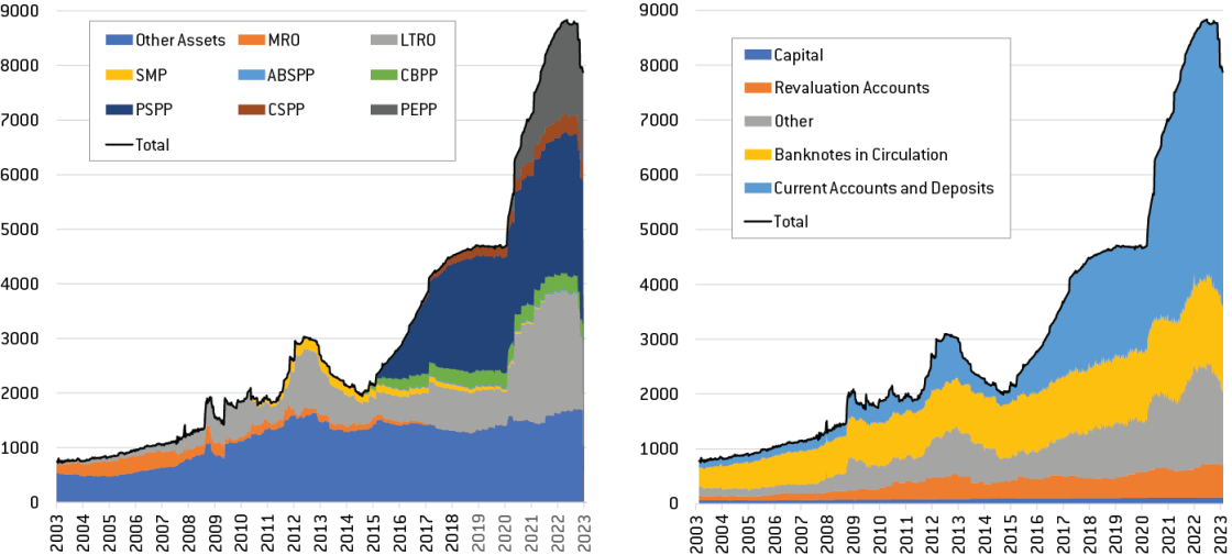
Source: Bruegel based on ECB’s Statistical Data Warehouse (SDW).

However, the combination of supply-side bottlenecks caused by the on-going COVID-19 pandemic in some regions of the world, the quick reopening of the euro area economy in 2021 and a strong increase in energy prices because of the war in Ukraine in 2022, led to a sharp increase in inflation in the euro area, up to double digits for the first time in four decades (Figure 3). The ECB decided it was time to tighten its monetary policy after a decade of accommodative policies. The most tangible form of this tightening has been the increase in ECB policy rates by 300 basis points (bps) between July 2022 and February 2023, the first increase since 2011 and the sharpest cumulative increase since the ECB’s creation in 1999 (Figure 2). Moreover, financial markets currently expect the ECB’s rates to rise further, by at least 100 bps by the end of 2023 ³ As can be inferred from future €STR pricing. See for instance: https://twitter.com/pietphc/status/1631266842005196801?s=20 .

But the ECB’s Governing Council also decided to adjust its balance-sheet policies. It first slowed and then stopped net asset purchases in the first half of 2022. After its December 2022 meeting, the ECB announced the end of full reinvestments and the start, scheduled for March 2023, of the unwinding of the asset purchases made under the Asset Purchase Programme (APP) ⁴ Given that the PEPP’s objectives were different, not only to fight deflationary risks but also to avoid fragmentation of sovereign bond markets in the euro area during COVID-19, the ECB announced when the programme was launched that maturing assets would be reinvested fully at least until March 2024. . Such a reduction of a central bank balance sheet through the unwinding of the portfolio of QE asset purchases is frequently referred to as ”quantitative tightening” (QT) ⁵ In some papers, the term QT is also sometimes used to characterise tapering episodes – i.e. episodes in which the central bank reduces its level of net asset purchases – or episodes of balance-sheet reduction through central bank loan unwinding, but in this paper we use QT in a narrow sense, only to characterise episodes of unwinding the portfolio of assets bought during QE episodes. .

QT is not the only way to reduce the size of the balance sheet of the central bank. Balance-sheet reduction can also take place endogenously through the repayment of loans made by the central banks to commercial financial institutions. In fact, though QT has just started in the euro area at time of writing, the reduction of the balance sheet of the Eurosystem has already been ongoing for a while. It has even accelerated in recent months since the recalibration of the ECB’s Targeted Longer-Term Refinancing Operations (TLTROs), with less advantageous terms decided in October 2022 (ECB, 2022a). This change encouraged banks to repay their loans to the ECB in advance. TLTRO repayments resulted in a substantial reduction of the size of the ECB balance sheet by almost €1 trillion between summer 2022 and February 2023 (Figure 1, Panel A).

Figure 2: ECB policy rates and short-term market rates (in %)

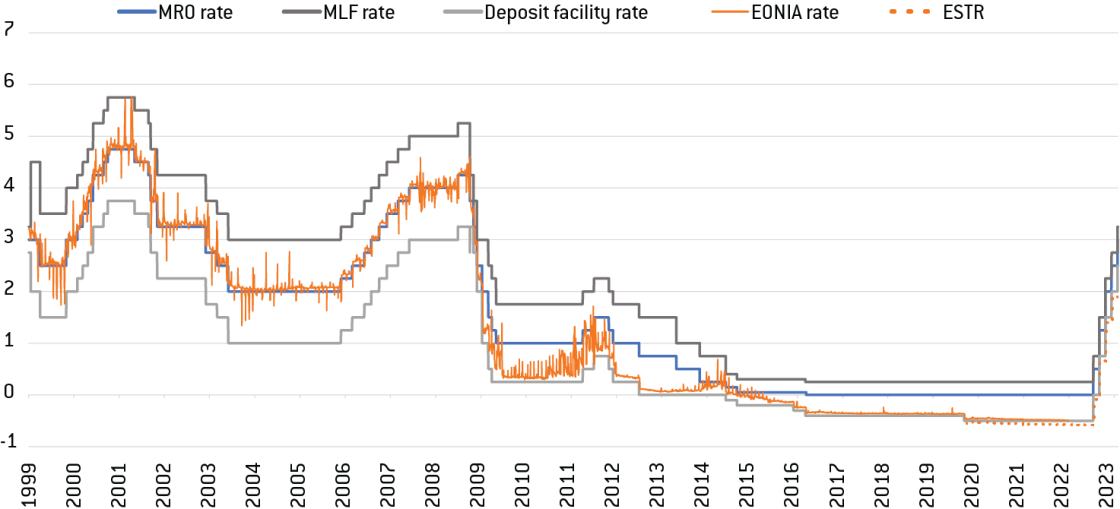
Source:  Bruegel based on ECB’s Statistical Data Warehouse (SDW).

What effects will QT in the euro area have? At this stage it is difficult to predict what will happen exactly because the empirical evidence from past experiences is very limited. QT has never been tried in the euro area, and historically there are only two main international experiences of QT to draw lessons from to guide policymakers: the US 2017-19 episode, during which the US Federal Reserve (Fed) reduced its asset holdings by around $750 billion (after a total increase of $3.7 trillion in the previous eight years); and the 2006-07 Japanese experience during which the Bank of Japan (BoJ) reduced its balance sheet from JPY 64 trillion to JPY 49 trillion (Blinder, 2010).

Most debates on the effects of QT are therefore not settled, but, based on the evidence available and on potential mechanisms at play, this paper discusses the following questions: what are the main reasons to do QT at this stage and are they all valid (section 2)? What could be the risks and possible side-effects of QT in the euro area in particular (section 3)? How can QT be done (section 4)? And how should the ECB do it to minimise potential risks (section 5)? 

2. Why do QT? Intended effects

2.1 The ECB’s rationale for starting quantitative tightening

The sharp increase in inflation since mid-2021 (Figure 3) has led the ECB to tighten monetary policy, like most other major central banks around the world. To do so, the ECB made it clear from the beginning that its primary tool to set the monetary policy stance would be its short-term policy rates, but it has also announced that it would use this occasion to reverse QE and to reduce the size of the Eurosystem’s balance sheet.

Figure 3: Euro area HICP inflation and its components (year-on year, in %)

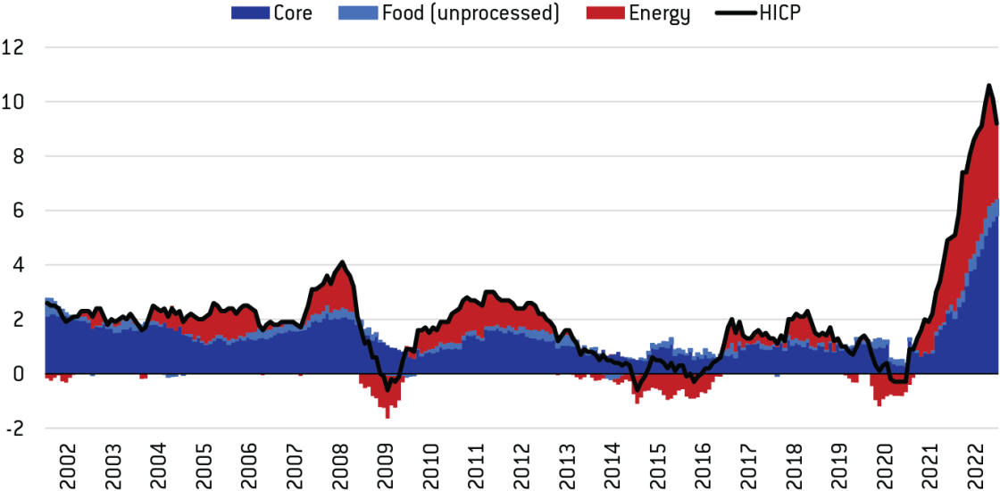
Source: Bruegel based on Eurostat.

But what is the ECB’s reason for this decision? Surprisingly, the ECB did not provide much explanation about why it had decided to launch QT when the decision was announced. During the ECB’s December 2022 press conference, following the meeting in which QT was formally adopted, President Lagarde minimised the significance of the decision by going as far as saying that, “there is no element of monetary policy stance, so to speak, associated with the reduction of the size of our balance sheet” (ECB, 2022b). She confirmed during the February 2023 press conference that QT was mainly seen as an “accessory instrument” (ECB, 2023b).

The accounts of the December 2022 meeting of the ECB’s Governing Council provided a few more hints on the logic behind the decision to start QT, explaining that the Council’s members see QT as a “necessary complement to the ongoing tightening of interest rate policy, signalling the Governing Council’s willingness to align all of its instruments so that they worked in the same direction”, that “accommodative liquidity conditions were no longer seen as required”, and that “announcing principles for normalising the Eurosystem’s monetary policy securities holdings [should] reinforce the impact of its rate hikes throughout the yield curve” (ECB, 2023a).

It looked like the ECB implicitly considered that reverting a policy often considered as ”unconventional” was an objective per se and that justifying it publicly was not really necessary. But, finally, the day after QT started, the ECB finally shed some lights on why it had decided to embark on this path. Schnabel (2023b), in a speech dedicated to the topic, listed three main reasons to do QT: “first, to regain policy space in an environment in which the current large volume of excess liquidity is not needed for steering short-term market interest rates; second, to mitigate the negative side effects associated with a large central bank balance sheet and footprint in financial markets; and third, to withdraw policy accommodation to support our intended monetary policy stance”, before explaining them in more detail.

At this stage, it is therefore crucial to review in detail these arguments and other arguments used to justify QT, to check their validity and to discuss thoroughly the possible risks that such a policy entails, in order to ensure that these risks are well taken into account by the ECB.

2.2 Main arguments in favour of QT in the euro area

 

There are three main sets of arguments to justify QT in the euro area: 1) economic arguments, 2) political economy arguments, and 3) legal arguments.

The first reason, cited but not really developed by the ECB, is that QT complements rate hikes by providing more monetary tightening. The simplest way to understand QT is first to assume that it is QE in reverse, and that its effects will be the same with a minus sign. This is in practice what most models used by central banks assume. This is the case at the Fed (Crawley et al, 2022) and at the ECB (as can be seen in the discussion of the Governing Council about the staff’s estimates in ECB, 2023a). And this is also what has been communicated to the public, for instance by ECB Executive Board member Schnabel ⁶ I. Schnabel during the Twitter #askECB event on 10 February 2023 stated that: “We would expect the effects of QE and QT to be largely symmetric”; see https://twitter.com/ecb/status/1624052843152900097. . If that is how QT works, the several rounds of QE in the US, the United Kingdom, Japan and the euro area in the last two decades should allow us to understand better the effects of QE and could thus help us estimate what the effects of QT could be. A back-of-the-envelope calculation based on estimates of the effects of QE in the euro area (Schnabel, 2021; Bundesbank, 2023), and assuming symmetry between QE and QT and linearity of the effect ⁷ These are very strong and probably unrealistic assumptions that are made for convenience, as we will see after. , suggests that a decline in the ECB’s asset holdings of €1 trillion could ultimately increase 10-year yields by between about 30 bps and 45 bps ⁸ Looking at overall effects on the economy, the ECB’s models suggest that reducing their asset portfolio by EUR 500 billion over 12 quarters would lower inflation by 0.15 percentage points and output by 0.2 percentage points over three years (Lane, 2023). . This extra tightening from QT is not negligible per se, but would represent only a small fraction of the effect resulting from the 300 bps increase in policy rates applied by the ECB from July 2022 to February 2023 – or even from the 400 bps that markets expect by the end of 2023.

Moreover, this back-of-the-envelope calculation probably overestimates the effect. Why? Because there are good reasons to believe that the effects of QE and of QT could be time-varying and state-dependent, as well as non-linear ⁹ For instance, the results of Alberola et al (2022) suggested that the effects of the ECB’s PEPP were non-linear. . The main reason is that some channels active during QE could be absent or attenuated during QT. For instance, the signalling effect of QE, which played an important role when purchases were made (Krishnamurthy and Vissing-Jorgensen, 2011) would probably be much less important during QT ¹⁰ By signalling effect, we mean that financial markets interpret QE as signalling lower policy rates ahead. . Similarly, QE played an important role in restoring market functioning during the global financial crisis and during the outbreak of COVID-19 in some countries. This effect would be nil in the absence of market stress. On the other hand, liquidity effects could be stronger during QT episodes than during QE (see section 3). Given that the current situation is very different from that prevailing when purchases were made, the effects of purchases and unwinding could then be asymmetric (as also highlighted by some Governing Council members during the December 2022 meeting, when discussing the ECB staff’s estimates). So, overall, QT might not play out exactly as QE in reverse.

This asymmetry is confirmed by the US 2017-19 QT experience: Smith and Valcarcel (2023) showed that QT tightened financial conditions, but its effects were not equivalent to those of QE in reverse. Similarly, the results from Wei (2022) suggested that a passive unwinding of a portfolio of $1 trillion could be roughly equivalent to an increase of the Fed funds rate of 13 bps if done in normal times, but that it would be equivalent to an increase of 34 bps during a crisis period.

A second argument often invoked to justify QT is the classical monetarist argument that a large amount of central bank money could result in rapid credit creation and boost inflation. QT would thus be needed to avoid that. This is not an argument brought directly forward by the ECB, but it might still be present in the back of the minds of some members of the Governing Council, given the reference to “liquidity” in their December discussion. In theory, the relationship between central bank money and broad monetary aggregates should be relatively stable because holding more reserves allows banks to provide more lending to corporations and households. However, empirically, the relationship has not been stable over time, and the major injections of liquidity by the ECB over the last decade have not resulted in a proportional increase in bank lending (Figure 4), or in broad money aggregates like M3.

Figure 4: ECB monetary base (M0) and bank lending to firms and households in the euro area since 1999

Panel A: M0 and bank loans (in EUR billions)                     Panel B: ratio bank loans/M0

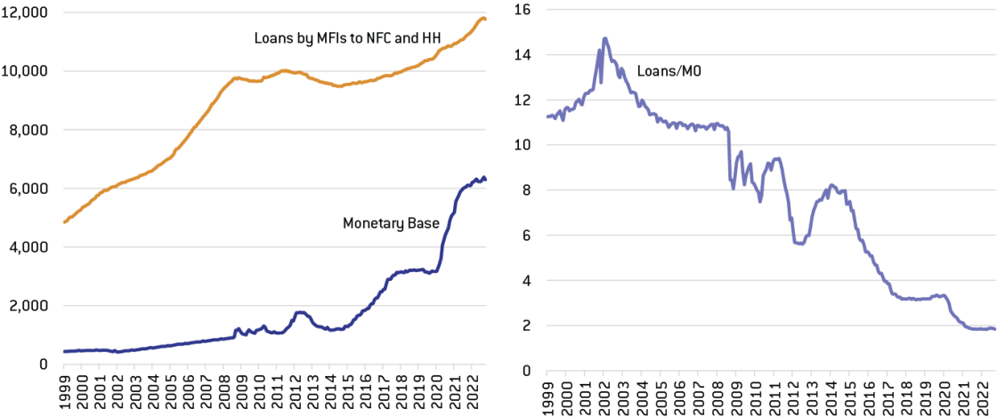
Source:   Bruegel based on the ECB’s SDW. Notes: M0: ECB monetary base, MFIs: monetary financial institutions, ie banks, NFC: non-financial corporations, and HH: households.

As discussed in more details in Claeys and Demertzis (2017), the main reason is that, in practice, bank lending in modern economies is largely determined by the level of interest rates and the corresponding demand for loans from firms and households, along with the credit risk evaluation of banks, their financial health and the prudential regulation affecting them. As a result, reserves at the ECB play a marginal, if any, role in the lending decisions of banks ¹¹ At the limit, and notwithstanding the fact that they have not be used in that way in recent decades, reserve requirements could be used to avoid an expansion of credit if they were to become binding. But this would mean that the ECB would implement QT to the point that it would fully drain excess reserves (i.e. up to 0) to provide a disincentive for credit creation. Such a reserve rationing seems highly far-fetched given that, at the time of writing, excess reserves stand at above EUR 4 trillion and central bank reserves may have become more needed than they used to (see discussion in section 3.1). . A high level of reserves should thus not prevent the ECB from tightening its monetary policy and from reducing lending in the euro area. In fact, the ECB Bank Lending Survey (BLS) for the last quarter of 2022 showed that the demand for loans is starting to fall strongly (Figure 5, Panel A) and that the rate hikes already implemented by the ECB are contributing very significantly to this trend (Figure 5, Panel B).

Figure 5: Net demand for loans in the euro area and contribution of the level of interest rates

Panel A: Net demand for loans (in %)                   Panel B: Impact of the level of interest rates (net %)

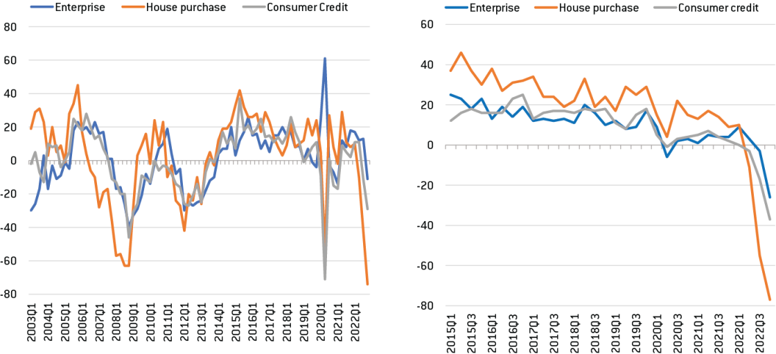
Source: Bruegel based on the ECB’s Bank Lending Survey, Q4 2022 (available on the ECB’s SDW). Notes: Net demand (in Panel A) refers to the difference between the percentage of banks reporting an increase in loan demand and the percentage of banks reporting a decline. Net percentage (in Panel B) is defined as the difference between the percentage of banks reporting that the level of interest rate has contributed to increasing demand and the percentage reporting that it contributed to decreasing demand.

A third reason to use QT could be to steepen the yield curve. One lesson from QE is that its effects are much more localised than those of policy rate changes, i.e. the price of the particular asset purchased is the one that is most impacted (see references in Krishnamurthy, 2022). If this local effect translates to QT, which is probably the case, this means that QT should mainly impact the medium- to longer-end of the yield curve (the weighted average maturity of the ECB’s PSPP holdings is around 7 years ¹² Source: https://www.ecb.europa.eu/mopo/implement/app/html/index.en.html. ). This can prove useful if the euro area risk-free yield curve is flat or inverted, as it is today (Figure 6), and if the ECB believes that short-term rate hikes are not transmitted enough to the rest of the curve to deliver the desired tightening (for instance, because markets believe that short-term rates will quickly go down in the next few years). But another important implication is that QT could be used not only to simply reinforce policy rate hikes, but also as an alternative way to tighten policy, as QT and hiking rates would provide different types of tightening ¹³ Another potential implication is that QT could also be justified from a financial stability perspective because a flat or inverted yield curve is generally considered to have a negative impact on banks’ interest margins. However, we do not believe that the ECB monetary policy stance should be determined by such financial considerations, given that the ECB (and the Single Supervisory Mechanism [SSM] in particular) has other tools at its disposal to deal with financial stability risks. .

Figure 6: Evolution of the euro risk-free yield curve since end of 2021 (in % per annum)

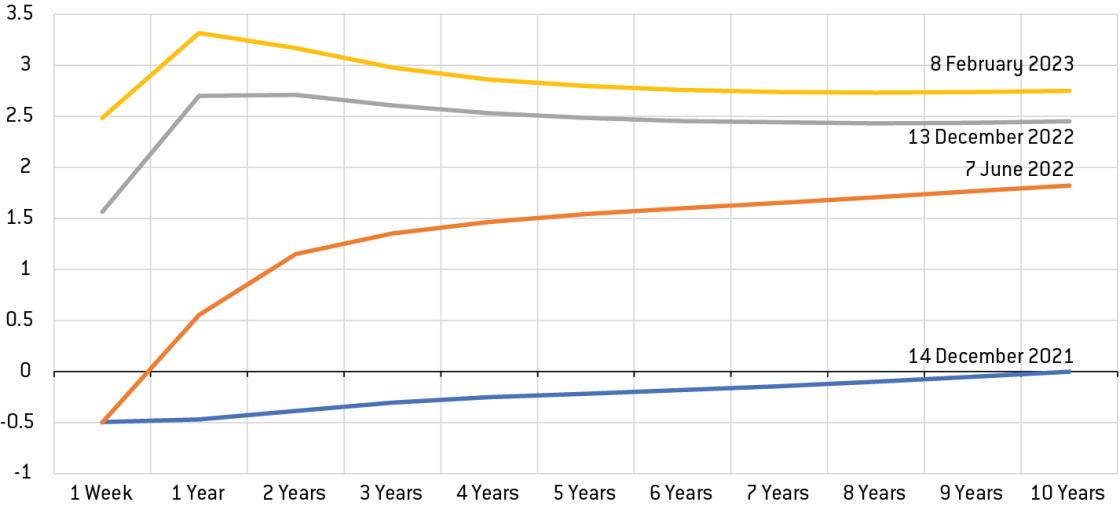
Source:   Bruegel based on Bloomberg. Notes: Euro OIS (overnight index swap) yield curves before selected ECB’s Governing Council meetings and at the time of writing (8 February 2023).

The ECB could thus fine-tune its monetary tightening by using different combinations of rate hikes and QT, if it wants it to be broad-based or sector-specific (e.g. to cool down a specific overheating sector like the housing market). Indeed, different sectors and economic agents are sensitive to different parts of the yield curve. In the US for example, mortgage rates and financing conditions for large companies are correlated with the long end of the curve, while consumer credit, car loans or SME bank loans are more correlated with short-term policy rates (Forbes, 2021). Sensitivities of particular sectors/agents to specific segments of the yield curve are possibly different in the euro area than in the US, and might also differ between countries of the monetary union ¹⁴ For instance, the share of mortgages that are contracted with a variable rate indexed against short-term rates varies widely between euro area countries, which means that the effect of an increase in short-term rates on households and the housing markets is very different across countries. , so this would need to be investigated thoroughly by the ECB. But, for instance, if the ECB wanted to keep tightening its policy without increasing the short-term end of the curve any further, in order to avoid removing too much monetary accommodation to sectors that are still vulnerable and that are more sensitive to short-term rates, it could decide to instead use QT to increase the long end of the curve more aggressively. However, a potential limit to this strategy is that this would probably mean unwinding a very large share of its portfolio rapidly to obtain a sufficient increase in the long-term part of the yield curve, if the effects of QT are smaller than those of QE, as discussed previously.

Another way to fine-tune its tightening using QT could also be to unwind the ECB’s various QE programmes at different speeds. Indeed, even if the PSPP represents the lion’s share of the ECB’s APP portfolio, the ECB also bought private assets through various purchase programmes (CBPP, ABSPP and CSPP). The objective of these programmes was often to revive or to boost specific markets to diversify sources of funding for euro area companies when investment was extremely low (either through corporate bonds or through bank loans which could be facilitated by the possibility offered to banks to issue more easily ABS or covered bonds). If these programmes have now fulfilled their objectives and outlived their usefulness, the ECB should consider unwinding these programmes more quickly than the PSPP, which would also allow the ECB to move away from the inherent credit risk borne by private assets.

Additionally, QT would be a prerequisite if the ECB wanted to go back to a lean balance sheet and to the corridor operational framework that prevailed before the global financial crisis, instead of the ample reserves/floor system that is now in place. There are several reasons to prefer a lean balance sheet (eg less exposure to commercial banks, insurance of having positive seigniorage profits which can protect the central bank’s financial independence, etc). However, there are also advantages to the current system ¹⁵ See Claeys and Demertzis (2017) for a more detailed discussion of the pros and cons of having a central bank with a lean or a large balance sheet. . What matters in the end is that the ECB controls short-term market interest rates that influence the rest of the yield curve, in order to transmit the monetary policy stance to the real economy. In that regard, the current system works very well: since 2015 the Euro OverNight Index Average (EONIA), and then the euro short-term rate (€STR) after 2019, have been very close to the ECB’s deposit facility rate (which de facto replaced the main refinancing operations (MRO) rate as the main policy rate in an ample reserve framework), and this spread has been extremely stable – in fact short-term market rates have been even much less volatile than in the previous regime (Figure 2). But, most importantly, going back to a lean balance sheet is probably impossible at this stage (see the discussion of the potential risks of QT in section 4).

A final economic argument is simply that it would be good to release back government bonds into the market. First, this would alleviate the scarcity issue affecting some euro area government bonds since the introduction of the ECB’s asset purchase programme, and which can be damaging for the good functioning of some markets that use them heavily as collateral, like the repo market (Arrata et al, 2020). Second, releasing bonds back into the market would also allow the ECB to regain policy space for the future. Generally, tightening policy only to be able to loosen it later is not a convincing argument, but in the specific case of QE, this argument could be more pertinent for two reasons: first, because, as we have seen, the effect of QT in non-stress times might be much smaller than that of QE and therefore it could be the right time to regain some margin of manoeuvre at a relatively low economic cost; and, second, because when the ECB designed the PSPP it introduced an issuer limit, which is currently equal to 33% for government bonds, to ensure the compatibility of the programme with the EU Treaties (see legal discussion below) ¹⁶ It is true that this constraint has been somehow relaxed with the ECB’s decision not to consolidate holdings from the PSPP and from the PEPP in 2020, but the ECB justified this by the different objectives of the two programmes and the particular nature of the PEPP (see detailed discussion in Claeys, 2020). . This limit could reduce the ability of the ECB to embark on QE (by reactivating and using the PSPP) in future crises, if holdings are not significantly reduced in the meantime. More generally, avoiding a ratchet effect could become particularly important if the ECB wants to be able to use QE regularly in the future: if QE becomes a conventional tool like policy rates, it needs to be able to go in both directions.

In addition to these economic arguments, there is also a strong political economy argument to be made to justify QT in the euro area. Since the beginning, the ECB has been uncomfortable with QE (which led to a delayed start compared to other central banks) because it sees it as blurring the separation between monetary and fiscal policies which could constitute a threat to its independence. Launching QT would then be a way to reduce the risk of fiscal dominance and reaffirm monetary dominance in the euro area. It would confirm that QE was not a permanent monetary financing of deficits (as it was sometimes perceived). This would also help ensure that inflation expectations remain well anchored, especially at a time when inflation is significantly above target.

Finally, in the euro area, there are also legal arguments in favour of QT because of the multi-country nature of the monetary union. In addition to complying with its price stability mandate, the ECB must also respect two main legal restrictions from the EU Treaties. First, the ECB is prohibited from financing directly Member States or EU institutions (Article 123 of TFEU). Second, like all EU institutions, the ECB should not act beyond its assigned competences and should thus be constrained by the proportionality and subsidiarity principles, i.e. it may only exercise the powers granted to it to the extent necessary to fulfil its mandate (Article 5 of the TEU).

The PSPP was legally challenged in Germany by EU citizens who believed these limits were not respected by the ECB. But the Court of Justice of the EU (CJEU) was consulted and considered that asset purchases constitute a legitimate tool of the ECB as long as there are “sufficient safeguards”. And it considered that the safeguards present in the PSPP ensured that the Treaties were respected. The safeguards were the following: no certainty about ECB buying and holdings, no disincentive for sound fiscal policy, no selective purchases, stringent eligibility criteria for the selection of assets, temporary and limited nature of the programme, and purchase limits (CJEU, 2018).

Among these safeguards, the one that matters most for our discussion on QT is the temporary nature of the QE programme, which could imply that QE has to be reversed once its goal has been reached. However, it does not mean that selling assets is compulsory as soon as the programme ends or that reinvesting is not possible when assets mature. The CJEU recognised that such actions can be necessary for the ECB to fulfil its mandate ¹⁷ The CJEU’s ruling states that: “The ESCB is thus entitled to evaluate, on the basis of the objectives and characteristics of an open market operations programme, whether it is appropriate to envisage holding the bonds purchased under that programme; selling the bonds is not to be regarded as the rule and holding them as the exception to that rule”, and that: “That means not only that the volume of purchases must be sufficient, but also that it may prove necessary — in order to achieve the objective pursued by Decision 2015/774 –– to hold the bonds purchased on a lasting basis and to reinvest the sums realised when those bonds are repaid on maturity” (CJEU, 2018). , but holding bonds for a lasting period should be justified by the ECB’s mandate and the ECB should explain clearly how this contributes to fulfilling its objectives. Holding the bonds to maturity, for instance, should be easily justified by the ECB by the fact that this is what was expected by financial markets at the time, and that failing to meet this expectation today could lead to a brutal adjustment in the short-term and also reduce the impact of asset purchases in the future. But, in the current economic conditions, the full and indefinite reinvestment of maturing assets would be more difficult to justify.

Similarly, the ECB should also make sure that its balance-sheet policies comply with the proportionality principle. In that regard, the CJEU could consider that the ECB’s policies are disproportionate if they are on a scale beyond what is needed to fulfil its mandate, e.g. sustained monetary accommodation when price stability is achieved, or worse, when inflation is above the target. In our view, these legal features do not necessarily mean that QT is absolutely compulsory to respect the provisions of the EU Treaties, but at minimum, not doing QT in the current situation would have to be justified very thoroughly by the ECB to comply with the safeguards mentioned by the CJEU in its 2018 ruling on the legality of the PSPP.

3. Possible risks and side-effects of QT

By starting the QT process in March 2023 for the first time in its history, the ECB is entering uncharted territory. This entails many risks. Some can be mapped out, but some are difficult to foresee at this stage, given our lack of familiarity with this policy. However, the first QT experimentation in the US from 2017 to 2019, during which the Fed reduced the size of its balance sheet by $750 billion over two years (Figure 7), represents our best chance to identify some of the potential side-effects of QT ¹⁸ The other main historical experience of QT in Japan in 2006-07 is much less documented and is quite different from today’s situation. Generally, the main takeaway is that QT was rushed in two main ways. First, it took place before inflation even went back towards its target in a durable way. And second, QT was done extremely quickly as the unwinding took place in a matter of months only, while QE had lasted for years (since 2001) and had been done at a much slower pace compared to more recent QE episodes (Binder, 2010). The significant differences in the whole QE/QT sequence but also in terms of economic situation with later episodes make it quite difficult to draw useful lessons for today from the Japanese experience. .

Figure 7: US Federal Reserve balance sheet (in $ billions)

Panel A: Assets                                                                   Panel B: Liabilities

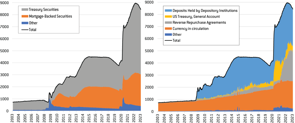
Source:   Bruegel based on FRED (Federal Reserve Bank of Saint Louis).

3.1 Scarcity of reserves and loss of control over short-term rates

One of the main lessons from the US experiment is that QT, and in particular the significant decline in central bank reserves associated with it, can lead to significant financial instability episodes. Indeed, this period was characterised by a severe stress episode in September 2019, which forced the Fed to put a halt to its first QT experiment (Copeland et al, 2021).

On 16-18 September 2019, the Fed temporarily lost control over funding costs in short-term money markets, which was shown by small spikes in the Effective Federal Fund Rate (EFFR, i.e. the interest rate depository institutions charge each other for overnight lending), and by large spikes in the Secured Overnight Financing Rate (SOFR, a broad measure of overnight Treasury repo rates), visible in Figure 8 (Panels A and B respectively). The spikes quickly faded when QT stopped, and volatility fully disappeared when asset purchases resumed. This highlights that markets have become more sensitive to the withdrawal of liquidity, which can lead to volatility in market rates ¹⁹ The evidence collected by Acharya et al, (2022) in the US suggested that this issue originates from the long periods of QE and the regime of ample reserves, which can create a state of liquidity dependence of the banking sector: banks change their behaviour during QE, but they do not adjust it when QE stops and when QT starts. As a result, the financial system can be more prone to liquidity shocks during a tightening cycle post-QE, which can lead to financial instability episodes. This means that QT can be risky, but also that it is probably necessary so that banks do not become too accustomed to abundant liquidity. .

Figure 8: Short-term interest rates in the US (in %)

Panel A: EFFR vs Fed rates                                     Panel B: SOFR vs Fed rates

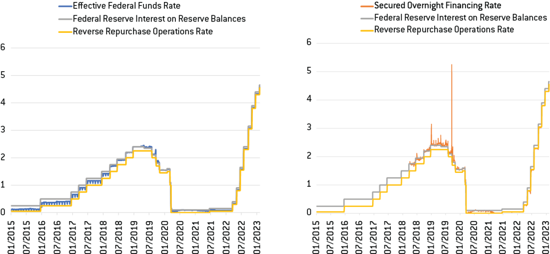
Source: Bruegel based on FRED (Federal Reserve Bank of Saint Louis). Notes: the EFFR is the short-term market rate at which banks and government-sponsored enterprises lend to each other in the federal funds market; the SOFR is a measure of the cost of borrowing cash against Treasury collateral using repo contracts.

What the Fed discovered on this occasion was that to function properly, the financial system structurally needs much more central bank reserves than before the global financial crisis. One of the main reasons is that financial institutions are required to hold much more liquid assets because the prudential regulations adopted after the financial crisis include strong liquidity requirements (such as the Liquidity Coverage Ratio). Another possible reason is that financial institutions may have learned their lesson from the crisis, and now understand the value of holding more liquid assets and have therefore adopted more prudent liquidity management practices. But a third possible reason, highlighted for instance by Greenwood et al (2016), is that the financial system already had a significant need for safe money-like instruments to function correctly before the crisis, but that, because the supply of such assets was insufficient, financial institutions turned to money-like debt securities provided by the private sector, in particular from the shadow banking sector, that were perceived as safe at the time. With the realisation that these securities were not really safe, the high demand for money-like instruments shifted back to ”real” money-like instruments, i.e. central bank reserves and short-term Treasury bills, which were then provided in large volumes. This meant that from this time onward, reserves would be needed in much larger quantities, as part of the policy response to the financial crisis. But since the end of net asset purchases in October 2014, reserves had actually been shrinking significantly and continuously (from $2.8 trillion to $1.7 trillion on the eve of the market-stress episode ²⁰ For simplicity, here, we define reserves as the combination of deposits of depository institutions at the Fed and of reverse repurchases agreements, as they represent a form of ‘reserves’ available also to non-bank financial institutions. ), because currency in circulation had grown endogenously with the size of the US economy (Figure 7, Panel B).

This shows why QT’s objective cannot be to return to a balance sheet similar to that prevailing before 2007, as too much QT could lead to frequent financial stability incidents. So how much QT is feasible? To calibrate how much can be done without risking loss of central bank control over short-term rates or without endangering financial stability, it is crucial to understand what the demand for central bank reserves is exactly, given that it is not directly observable ²¹ If lower reserves translate only into a higher but stable spread with the relevant policy rate, this would be less of a problem but would have to be taken into account when calibrating monetary policy rates. .

Since the aforementioned market-stress episode, central banks have started to work on this issue. In the US, Fed researchers Lopez-Salido and Vissing-Jorgensen (2022) attempted to model the demand for reserves to estimate the quantity that would be compatible with a low spread between the EFFR and the Fed’s Interest on Reserves Rate (IOR) ²² The operational frameworks of the Fed and the ECB differ but the IOR can broadly be considered as the equivalent of the deposit facility rate of the ECB. at the end of 2022. Their results suggest a number between $ $2.8 trillion and $3.5 trillion, meaning that feasible QT in the US would be as small as $2 trillion. In the UK, the Bank of England (BoE) chose another path to gauge how much reserves are needed, and simply asked its main counterparties what their needs are and why they hold reserves. As expected, regulations requiring banks to hold liquid assets play an important role (Hauser, 2019). These conversations with financial institutions suggested that the level of needed reserves in the UK is around GBP 150-250 billion, out of a total amount of reserves standing at around GBP 900 billion at the time of writing. In the euro area, ECB researchers (Åberg et al, 2021) suggested that the short-term market rate (i.e. the EONIA/€STR) could start increasing sharply if excess reserves fall below €1 trillion. This seems relatively low compared to the Fed’s estimates, or even to the actual level of reserves prevailing during the September 2019 episode – i.e. around $1.7 trillion – for balance sheets that are roughly of the same size (in their own currencies). In any case, these numbers should be taken with caution given the very high uncertainty surrounding these estimates.

Finally, if, unfortunately, QT is mis-calibrated and the level of reserves becomes too small, the liquidity insurance toolkit of the central banks will need to play a crucial role. That is why the Fed introduced a new Standing Repo Facility (SRF) in July 2021 to provide liquidity when needed to avoid spikes in money markets, even if it has not been tested yet. On its side, the BoE has announced that it will launch a new Short Term Repo (STR) facility to ensure that financial institutions can have sufficient access to liquidity during and after QT, and that short-term market rates remain close to its policy rate, but also to be able to make future decisions about QT independently of the implications for the supply of reserves (Hauser, 2019; BoE, 2022c). The ECB, however, has not discussed this issue for the moment.

3.2 Impact on government bond markets and possible ripple effects

As discussed in section 2, there are good reasons to think that the effects of QT on the economy could be relatively muted, or at least smaller than those of QE. However, the uncertainty is high because QT has never been tried in the euro area. It has been tried in the US in the past and is now in full swing again in the US, as well as in the UK and in Canada. But the effects in the euro area could differ, in part because of the euro area’s multi-country nature and its different institutional and legal architecture.

If the objectives of QT are to provide extra tightening by steepening the yield curve – in other words to increase directly long-term rates – and to reduce the scarcity of government bonds in financial markets, the other side of the coin is simply that bond prices should go down and sovereign bonds might become too abundant. There could be several risks associated with these movements, if not managed carefully.

One of the main risks related to QT is that markets could struggle to absorb sovereign bonds if they were released by the Eurosystem too quickly. In the euro area, the specific risk most often discussed ²³ See e.g.: https://www.economist.com/finance-and-economics/2022/11/24/why-europe-i…. is that QT could lead to an unwarranted increase in the spreads of some countries versus German yields and a fragmentation of sovereign bond markets, which could lead to a too-strong tightening in some countries, incompatible with the desired monetary stance of the ECB (Claeys et al, 2022) and possibly threatening the sustainability of public finances (Alberola et al, 2022). The reason for this fear is that if asset purchases have contributed to reducing spreads between countries, spreads could increase quickly with QT (Alberola et al, 2022). As discussed previously, this will not necessarily be the case, as QE and QT effects are probably asymmetric. Nevertheless, given the high uncertainty and the high stakes involved, this risk should be taken seriously and monitored carefully.

As of today, despite a significant increase in the spreads of countries with debt-to-GDP ratios above 100% when markets started expecting ECB rate increases and the end of net asset purchases after September 2021 (Figure 9, right panel), their recent levels remain relatively moderate compared to previous peaks (e.g. at the beginning of the COVID-19 outbreak, at the height of the tensions between the Lega-M5S Italian government and the European Commission in 2018-19, not to mention the extraordinary levels reached during the euro crisis, Figure 9, left panel). Moreover, the establishment of the Transmission Protection Instrument (TPI) by the ECB on 21 July 2022 reassured markets that the ECB would continue to honour its 2012 promise to do “whatever it takes” to ensure the integrity of the monetary union and to counter unwarranted market dynamics that threaten the smooth transmission of monetary policy in the euro area. Since the announcement of the TPI, spreads have declined towards relatively moderate levels (not far away from their historical averages since the creation of the euro), despite the ECB’s recent announcements on the normalisation of its balance sheet, and the fact that these were generally more hawkish than what was expected only a few months ago.

Figure 9: 10-year interest rate spreads vs Germany in selected countries (in %)

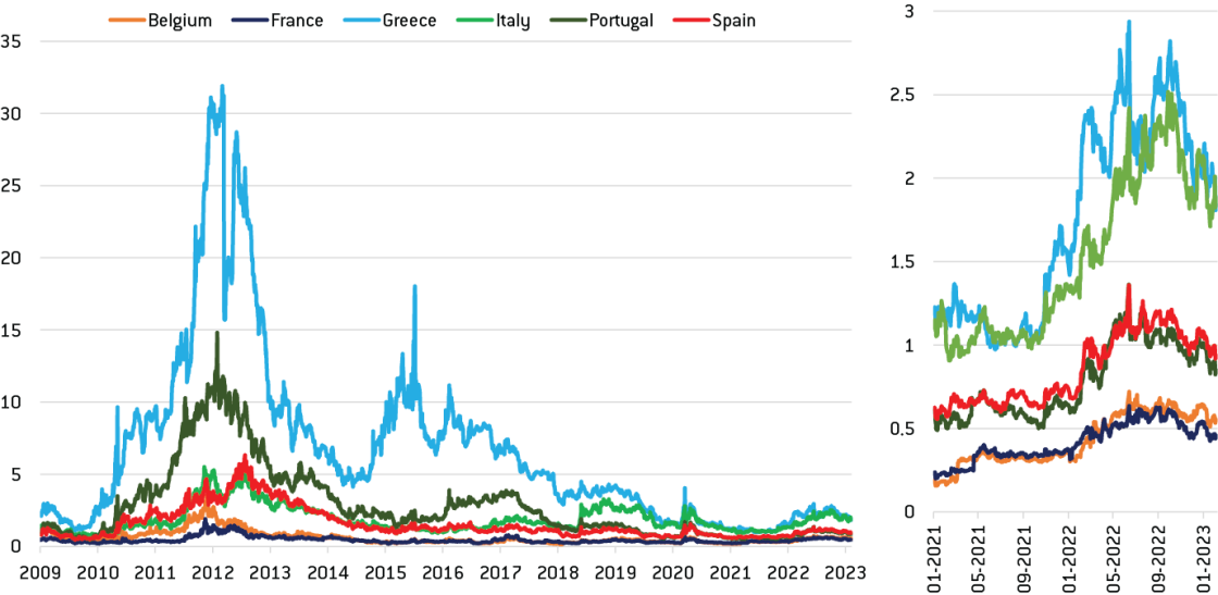
Source:   Bruegel based on Bloomberg. Note: countries selected all have currently a debt-to-GDP ratio above 100%.

Furthermore, as QE starts to affect yields when markets start expecting the policy and at the time of its announcement, QT possibly works in the same way. Given that markets already expect a significant amount of QT to take place in the next years, it is therefore possible that the effects of QT on yields have already materialised to a great degree, and that its actual implementation will not increase yields (and spreads) much further, unless QT is larger than currently expected, i.e. around €500 billion between now and the end of 2024 (ECB, 2023d).

Another possible risk could arise from the impact of a too-rapid change in bond prices on the holders of these assets, which could lead to financial instability. The experience of the UK in September 2022 is very instructive in that regard. The presentation of the UK’s government “mini-budget”, characterised by large tax cuts and subsidies and no realistic plan to finance them, on 23 September 2022 led to a very rapid increase in long-term yields. As a result, British pension funds were forced to offload a large number of gilts at distressed prices, triggering margin calls on derivatives designed to protect the funds against large movements affecting gilts. This threatened the solvency of some of the funds and forced the BoE to postpone its plans to start QT and, on the contrary, to intervene in the government bond market temporarily to end the market panic ²⁴ For a detailed explanation of what happened in the UK in September 2022, see for instance: https://www.ft.com/content/038b30c3-f550-4cc0-93ed-9154021d6ee2. .

To be perfectly clear, this episode was not triggered by QT, but by the presentation of a worrying fiscal plan. However, we mention it, first, because it is a good example showing that abrupt changes in the price of government bonds (whatever their underlying origin) are not desirable from a financial stability perspective. A perfectly identical episode might not occur in the euro area if the mechanism at the heart of this crisis was specific to the UK (e.g. because of the specific regulations affecting UK pension funds), but it highlights that a quick change in the yield/price of sovereign bonds that are widely used by many actors can lead to unforeseen market stress coming from any corner of the financial sector. To prevent such situations from arising, QT should be designed explicitly to avoid large swings in government bond prices. A second lesson is that, in these situations, central banks need to adjust their policies very quickly. Given the legal constraints surrounding the ECB and the difficulties of having to deal with 19 different government bonds ²⁵ There are 20 members of monetary union since Croatia joined in January 2023, but the ECB has not yet purchased any Croatian bonds at this stage, given that net asset purchases stopped before its entry. , compared to the tight and simple relationship between the BoE and the UK Treasury (or between the Fed and the US Treasury), it might not be as easy for the ECB to take quick decisions involving government bond purchases to end market stress. And because changing course is not as easy for the ECB as for other major central banks, it needs to be much more careful in its decisions ex ante.

Overall, members of the ECB Governing Council advocating for a gradual QT seem primarily concerned about the risks associated with the unwinding of the bonds sitting on the asset side of the ECB’s balance sheet (ECB, 2023a ²⁶ During the ECB’s December 2022 meeting, some members of the Governing Council feared that: “too fast a pace of reduction could lead to the re-emergence of bond market fragmentation” (ECB, 2023a). ; Hernández de Cos, 2022). These risks should not be treated lightly: the transmission of monetary policy could be impaired in some part of the monetary union, public finances could be endangered in some countries, and large swings in government bonds’ prices could trigger financial instability episodes. However, at this stage these risks appear to be mostly under control thanks to the ECB’s TPI. In addition, the US experience suggests that critical risks could also arise from unwinding the liability side. If this is the case, it does not matter if the reduction in bank reserves come from QT (i.e. the unwinding of the QE asset portfolio) or from the unwinding of the ECB’s large lending operations (TLTROs). In that respect, it is important to note that, as of early February 2023, reserves have already decreased by €700 billion since their peak in November 2022, and the full reimbursement of TLTROs could reduce them by an additional €1.2 trillion over the next year (Figure 1, Panel A) ²⁷ The last TLTRO will mature on 18 December 2024, but banks could end up reimbursing the funds much earlier than that. . One important lesson for the ECB is that it should be at least equally worried about this problem as about spreads when designing its QT programme.

4. How can QT be done?

4.1 Main options and crucial parameters to take into account

To make it simple, there are four main options to implement QT. These possibilities are not all mutually exclusive: they can in some cases be combined or implemented sequentially depending on the objective pursued (degree of tightening desired, willingness to regain quickly margins of manoeuvre for later, etc, as discussed in section 2). We present them here, from the more to the less aggressive variety, and discuss their main general pros and cons (those specific to the euro area are discussed in the next section):

1. Active sales of the assets bought during QE. The main advantages of this option are that the central bank controls perfectly the pace of the balance-sheet reduction, that the unwinding can be quick and that, if the economic situation warrants it, a stronger monetary tightening effect can be expected compared to other options. The main drawback, as discussed in the previous section, is that this “active QT” entails some significant financial stability risks.
2. Fully passive unwinding of purchased assets: the central bank does not reinvest the proceeds from maturing assets and lets the balance sheet decline mechanically. The main advantage of this option compared to option 1 is that financial risks would be less, that the timing of redemptions would be well-known by market participants and also that this is probably the option that markets expected when QE was launched. One drawback is that the reduction pace could be quite irregular because it would depend on the level of monthly redemptions, which are not necessarily perfectly linear (see e.g. the ECB’s expected monthly redemptions in 2023 in Figure 10).
3. Partial reinvestment of maturing assets: the central bank caps the reduction of its balance sheet per month. In addition to being even more gradual (which can be a desired characteristic if not much tightening is needed from QT) and less risky than the previous option, the main advantage is that the balance sheet reduction would be regular and might be easier to communicate to the public, because it would be symmetric to the way asset purchases were implemented.
4. Full and indefinite reinvestment of maturing assets while required reserves and currency in circulation increase with the size of economy and eat up excess reserves (even if this slightly stretches the definition of QT as the reduction would only happen in GDP terms). The main drawback of such a strategy is that balance-sheet normalisation could be very slow due to the combination of large balance sheets and low foreseen growth rates in advanced economies. This could make the use of QE more difficult in the near future or could risk creating a ratchet effect. Moreover, the tightening effect would probably be very small if not totally muted. The main advantage is that the financial stability risks would be largely absent.

Interestingly, most central bank balance-sheet normalisations of the twentieth century were achieved by keeping balance sheets nominally stable and by shrinking them as a share of GDP (Ferguson et al, 2015). As a result, these reductions were often protracted: for instance, after the large expansions due to war financing by central banks during the Second World War, the unwinding (in GDP terms) which started at the end of the 1940s extended up to the late 1960s in many countries. In fact, apart from the recent experiences in US and Japan, there are only very rare historical examples of balance-sheet reduction through a nominal contraction of assets, and when it was done it was not done through QT ²⁸ Sweden’s Riksbank reduced twice the nominal size of its balance sheet in the last three decades. First, in 1993-98, when Sweden abandoned its fixed exchange rate regime, the central bank reduced significantly its foreign currency reserves; and second, after 2010 the Riksbank’s assets shrunk quickly when the loans made to commercial banks during the global financial crisis expired (Ingves, 2020). Similarly, in 2012-14, the ECB’s balance sheet declined quickly when commercial banks started reimbursing longer-term refinancing operations (LTROs) contracted in 2010-11. .

In addition to choosing between these four main strategies, and/or how to sequence them, there are other parameters to consider when designing a QT programme:

• First, the pace of the unwinding of the asset portfolio, in particular if the central bank opts for asset sales or for a partial reinvestment cap: the pace will mainly depend on the exact reason why the central bank wants to do QT, but will also have to consider potential trade-offs with financial stability risks.
• Second, the interactions and the sequencing with other monetary policy tools: a consensus on the normalisation sequencing has emerged among central bankers: start by tapering QE, followed by a period of reinvestment of maturing assets, then policy rate hikes, and finally QT (in its various form). But other sequencing could have been considered: QT could have preceded rate hikes. This could have had some clear advantages: if its tightening effect is smaller than that of rate hikes it could have been a way to start tightening more smoothly, even before inflation reappeared, and it would have had the additional advantage of limiting temporary losses by central banks during the rate increase ²⁹ Central banks are not profit-maximising institutions and losses do not really matter for the conduct of monetary policy, but positive profits ensure the financial independence of central banks and thus facilitate their operational independence from a political perspective. . The most common reason given to justify the current consensus sequencing is that there is more certainty about the effects of rate changes than of QT. However, Forbes (2021) speculated that the Fed chose this sequencing to push back QT as much as possible because of the bad memories from the ”taper tantrum” episode of 2013. And now, because the US QT experience is the main one to draw lessons from, all other central banks safely copy the Fed sequencing, without really looking in depth into the various pros and cons of different possible sequencings.
• Finally, all other considerations discussed previously in section 2 should also be taken into account in the design of the QT programme, and in particular the desired size of the balance sheet in the long run, which should play an important role.

4.2 State of play of QT in major central banks as of February 2023

The Fed published its ”principles” for reducing its balance sheet as soon as January 2022 (Fed, 2022a). This was followed by a more detailed ”plan” in May 2022 (Fed, 2022b). QT started the following month when the Fed allowed some securities to mature without reinvestment up to monthly redemption caps. In accordance with its initial plan, the Fed set its cap at $47.5 billion per month (split between $30 billion of Treasuries and $17.5 billion of Mortgage-Backed Securities), before doubling it to $95 billion per month after three months (with a $60 billion-$35 billion split). As a result, the Fed’s asset holdings were already reduced by more than €500 billion between June 2022 and February 2023 (Figure 7, Panel A), a much faster pace than during the 2017-19 QT episode.

The BoE published its principles on how to tighten monetary policy as early as August 2021 (BoE, 2021), in which it explained the sequencing of the monetary tightening and the reasoning behind it. It also contained two clear criteria on when it would start QT: a policy rate above a certain level (in order to be able to reverse significantly its rate hikes if QT had a stronger effect than expected) and a normal functioning of markets. In February 2022, the Monetary Policy Committee (MPC) decided to launch QT before the end of the year (BoE, 2022a). In May 2022, the BoE provided details to markets about the future sales of corporate bonds which would be starting in September (BoE, 2022b). In August 2022, the MPC agreed that it would vote on a twelve-month reduction in the stock of gilts comprising both maturing and sales, and it would do so every year as part of an annual review (BoE, 2022c). In September 2022, when its policy rate reached 2.25% and market conditions were judged appropriate, the MPC decided to reduce its holdings of UK government bonds by GBP 80 billion during the next 12 months through maturing but also sales (BoE, 2022d). The unwinding of corporate bonds started on 27 September 2022, but the gilt sales started only on 1 November 2022, postponed because of the September mini-budget market stress that led the BoE to implement temporary purchase of gilts (BoE, 2022e).

Other central banks around the world have also started to implement QT and have chosen different strategies to do so. The Bank of Canada and the Reserve Bank of Australia have opted for passive QT, the Reserve Bank of New Zealand has opted for active sales, while Sweden’s Riksbank has decided to do QT through partial reinvestment (OECD, 2022).

 

4.3 What is the plan of the ECB concerning QT at this stage?

Since December 2018, the ECB’s Governing Council had announced clearly the sequencing of its future policy normalisation, which follows exactly the Fed’s rulebook: QE tapering, reinvestment of maturing assets, rate hikes and finally QT ³⁰ All the ECB’s press conference introductory statements during this period (and until October 2022) included a version of the following sentence: “The Governing Council intends to continue reinvesting, in full, the principal payments from maturing securities purchased under the APP for an extended period of time past the date when it starts raising the key ECB interest rates and, in any case, for as long as necessary to maintain ample liquidity conditions and an appropriate monetary policy stance.” . After having already increased its key rates by 200 bps since July 2022, the ECB announced in December that it intended to unwind its QE programme at a “measured and predictable pace” by reducing its APP holdings by € 15 billion per month on average from March to June 2023 – in other words through a partial reinvestment strategy. At the time of writing, the ECB had not announced yet what it will do after June 2023, apart from the fact that “the pace [of QT] will be determined over time” (ECB, 2022b).

How did the ECB come up with the €15 billion per month number? President Lagarde replied to that question during the December 2022 press conference: because “it represents roughly half the redemptions over that period of time” (ECB, 2022b). Indeed, redemptions will average €32 billion per month between March and June (Figure 10). This answer, along with the discussions during the Governing Council meeting 31 See footnote 26. , suggests strongly that the ECB’s QT pace calibration is more driven by financial stability considerations than by its tightening effect.

As promised in December, the ECB also released additional technical details about its QT policy after its February 2023 meeting (ECB, 2023b and c). Two features are worth highlighting in our view. First, the ECB plans to distribute the reduction proportionally to the redemptions (meaning the PSSP should decline on average by around €12 billion per month and the private sector programmes by €3 billion in total in the March-June period). Second, the ECB plans to tilt slightly the partial reinvestments of its corporate bond purchases (in the CSPP) towards issuers with better climate performance.

Figure 10: Expected monthly redemption amounts for the APP (in EUR billions)

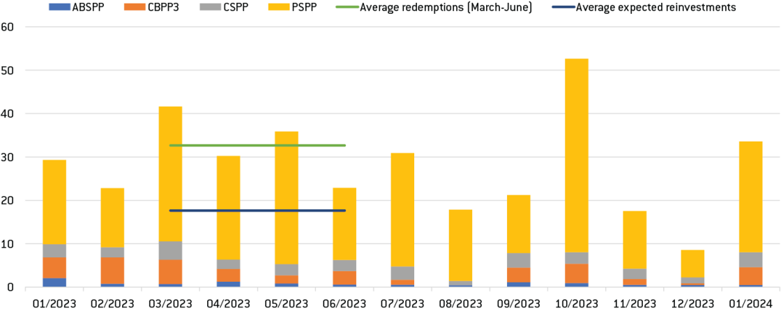
Source:   Bruegel based on ECB.

5. Conclusions: what should the ECB do?

The ECB started its QT policy on 1 March 2023, and has not yet made any commitment about how it will proceed after the first four months. This means that there still exists significant room for manoeuvre to improve and recalibrate QT if needed. Given what we have learned so far about the effects and potential risks related to QT, what do we think the ECB should do?

All in all, we believe that QT is largely justified in the euro area, even if there are good and bad reasons to do QT. In the end, the economic case to do QT is relatively weak. QT can probably provide some additional tightening to rate hikes, but its effects are possibly small and anyway uncertain. Besides, it is probably not much needed as interest rates hikes (by 300 bps already and possibly by 400 bps by the end of the year) should already have a very restrictive effect in the medium-term. One of the main benefits of QT on that front is that it could be used to steepen the yield curve, which could allow the ECB to fine-tune its tightening. Combining short-term policy rate changes and QT could either make its tightening more broad-based if that is needed, or, on the contrary, the ECB could use QT to target specific sectors/agents, or even insulate others by using QT more forcefully to increase the long-end of the curve, while reducing the pace of policy rate hikes ³² One possible argument against this type of fine-tuning is that it would possibly require more knowledge than currently available on the effects of QT. Another reason is that it could put the central bank in the business of resource allocation more explicitly, for which the ECB does not have an explicit mandate.  (which in our view would be a good idea in any case in order to take the time to observe the effects of past rate hikes on the economy at this stage). On the contrary, advocating for QT because there is too much liquidity, which could lead to too much lending and ultimately boost inflation, is probably not a good reason. And constraining lending further would in any case probably not be needed as the demand for loans is already falling quickly in the euro area as a result of the ECB’s large rate hikes.

Ultimately, the most compelling reasons to do QT in the euro area are therefore mainly political and legal. Doing QT finally confirms that QE was not a permanent monetary financing of deficits, as it has been sometimes perceived, which could help ensure that inflation expectations remain well anchored. Moreover, QT will also confirm that QE was temporary and proportional, and thus complied fully with the limits assigned to the ECB by the EU Treaties. In that regard, QT will make QE more conventional and will facilitate its future use from a political and legal perspective. And in practice, QT will also help the ECB regain quickly some margin of manoeuvre if QE needs to be used in the near future (this is particularly true in the euro area, where asset purchases are more constrained) ³³ The possibly limited effect of QT in good times reduces its attractiveness as a tightening tool, but also reduces the economic cost of using it to regain some policy space (contrarily to rates). .

If QT is justified, how should the ECB do it? In general, given the large uncertainty surrounding QT, the ECB’s lack of experience in this field, and the potential risks QT entails, the ECB’s approach should be based on the precautionary principle. The ECB should be extremely flexible, it should carefully monitor the direct effects of QT on financial conditions, learn more generally about the magnitude of its impact, and be ready to amend or reverse it if there are unintended results (in particular in the case of market dysfunction). But the ECB should also be ready to accelerate QT if everything goes well and the benefits of the policy outweigh its potential costs more than expected ³⁴ Being flexible however does not mean that the ECB should be vague about its future policy. On the contrary, the ECB should provide a state-contingent roadmap to markets to avoid them being surprised by policy adjustments. .

What particular features of its plan should the ECB revise? The moderate pace of QT decided by the ECB is probably a good initial strategy, especially given the concomitant large rate hikes. Outright asset sales, like those implemented by the BoE, would entail some major financial risks and are not necessary in the euro area. One reason is that the weighted average maturity of assets held by ECB is relatively short, with around seven years remaining on average for sovereign bonds, while the maturity of the gilts held by the BoE is almost twice as long (OBR, 2021). Waiting for assets to mature is thus less of a problem for the ECB. On the other side, reducing the portfolio of QE assets only in GDP terms, as was done often during the twentieth century, would be a safe option from a financial stability perspective, but would probably be too slow to regain some QE policy space quickly before the next crisis (and could be legally challenged if not well justified). Therefore, partial reinvestments appear to be the right option at this stage. We believe that the ECB is right to start small to observe the effects of QT on yields and spreads. If risks do not materialise, the ECB could then accelerate QT and, at some point, move towards a fully passive unwinding of QE assets, which would be roughly in line with what markets have been expecting, until its balance sheet reaches its desired size compatible with financial stability. Given that markets already expect a reduction of the ECB’s asset portfolio by around by €500 billion by the end of 2024 (ECB, 2023d), a reduction of this scale should probably not rock yields and spreads.

However, the ECB should change its current plan concerning the distribution of QT across its various programmes. We believe there is no reason for the ECB to hold private assets if the associated markets are functioning normally. The ECB should thus accelerate the end of its private programmes (ABSPP, CBPP and CSPP), even possibly by considering assets sales. Two additional advantages would be that: 1) the ECB would not need to find a satisfactory way to tilt its corporate bond reinvestments towards greener assets, and 2) if it felt the need to do so, the ECB could increase the pace of QT by increasing the speed of the unwinding of its private programmes, without increasing the risks related to the functioning of euro area sovereign bond markets.

But as we have seen QT also entails some risks, how could the ECB be better prepared to deal with risks, and in particular with financial risks? The ECB is careful to avoid any disruption in the functioning of financial markets, which is obviously a good thing. Some members of the Governing Council are particularly worried about the re-emergence of a fragmentation risk due to QT. Such a possibility should not be treated lightly, but for the moment this risk seems to be under control thanks in large part to the ECB’s TPI, which the ECB should not hesitate to use if needed ³⁵ To deal with this risk, as a first line of defence, the ECB also has at its disposal the flexible reinvestment of maturing assets from the PEPP which is expected to continue until end of 2024 (given the ECB’s initial commitment on the PEPP it makes sense to avoid changing this to avoid any time consistency issue which could reduce the impact of asset purchases in the future). . However, given that the access of countries to the TPI relies, at least partly, on their compliance with EU fiscal rules, the best way to reinforce the credibility of this tool and thus to reduce the fragmentation risk would be to find an agreement on the reform of the EU fiscal framework along the lines proposed by the European Commission on 9 November 2022 (European Commission, 2022) ³⁶ See for instance the explanation and an assessment of the proposal by Blanchard et al (2022). . The European Parliament could play a crucial role by pushing the other EU institutions to reach an agreement before the end of 2023, so that the old flawed fiscal rules are not reinstated in 2024.  

In addition, the ECB should also think more carefully about the risks that could arise from the liability side of its balance sheet. Indeed, when designing its QT policy and in particular when deciding about its pace, the ECB should be sure to avoid creating any reserves scarcity, which can lead to market stress episodes, as highlighted by the US September 2019 episode. In that regard, the ECB should be extremely careful about the interaction of QT with the balance-sheet reduction resulting from the unwinding of its TLTROs, which the ECB does not fully control. With central bank reserves around €4.2 trillion, required reserves at €200 billion, demand for excess reserves at EUR 1 trillion, a (conservative) buffer of another trillion, and TLTROs that could decrease quickly by €1.2 trillion, a simple back-of-the-envelope calculation suggests that only €800 billion of QT could be feasible, possibly less if the demand for reserves is more similar to that in the US (but a bit more than the €500 billion that markets currently expect by the end of 2024).

The ECB should investigate the question in more depth and by all possible means (using models like the Fed, but also surveying counterparties like the BoE) so that the Governing Council can have a clear, and official, view on how much QT is feasible exactly before such a problem could arise ³⁷ Apart from the pre-cited working paper by the ECB’s staff (Åberg et al, 2021), which represents the view of its authors and not those of the ECB’s Governing Council, as the usual disclaimer states, we could not find any reference to how much QT is feasible in the euro area in the ECB’s official documents (press conference, press release, accounts of the meetings, speeches, etc). , and on what should be the long-term size and composition of its balance sheet. In particular, even if Executive Board member Schnabel (2023a) already hinted at “a larger steady-state balance sheet, potentially including a structural bond portfolio”, the scheduled review of the ECB’s operational framework to control short-term market rates is only expected to be concluded by the end of 2023. In our view, this should be brought forward to bring some clarity to the market as soon as possible ³⁸ As stated by President Lagarde during the December press conference: “By the end of 2023, we will also review our operational framework for steering short-term interest rates, which will provide information regarding the endpoint of the balance sheet normalisation process” (ECB, 2022b). .

In practice, to keep some sufficient buffers, the ECB could think about switching at some stage to a variant of the fourth option discussed in section 4.1: after reducing its balance sheet to a lower but safe enough level, the ECB could reduce further its direct bond holdings, while keeping its balance sheet nominally constant by replacing maturing assets gradually with open market operations.

If, nevertheless, central bank reserves become too scarce, what liquidity tool should the ECB use to deal with stress in short-term money markets and an unwarranted increase in its operational target market rate, the €STR? After its 2019 stress episode, the Fed announced in July 2021 the creation of a new Standing Repo Facility (SRF) to avoid pressures on overnight rates. The BoE has also announced the creation of a new Short Term Repo (STR) facility to ensure that short-term market interest rates remain close to its policy rate during QT. Does the ECB also need a new lending facility? The ECB already has at its disposal a toolbox of traditional lending operations to inject liquidity: 1-week MROs, 3-month LTROs, both at fixed rate and full allotment since 2008, and its marginal lending facility (MLF) which offers overnight credit to banks and which rate is 75 bps above the deposit rate and 25 bps above the MRO rate. These tools, which are less central when reserves are extremely abundant due to QE and TLTROs, should become crucial again. Therefore, the ECB does not need a new tool in our view. However, to be sure to control short-term market rates more tightly, it could consider reducing the spreads between the MRO, the MLF and the deposit facility (DF) rates, for instance by reducing the DF-MRO spread from 50 bps to 25 bps, which would bring the DF-MLF spread to 50 bps instead of 75 bps ³⁹ For instance, at the BoE, the STR (the equivalent of the MRO) is priced at the same rate as the Reserves Accounts (the equivalent of the DF), while the Operational Standing Facility (the equivalent of the MLF) is only priced 25 bps above. .

To conclude, even if there are good reasons to do QT in the euro area at this stage, it does not exempt the ECB from explaining what the main risks related to it are, how it will take them into account to try to avoid them, how it will deal with them if they materialise, what main potential trade-offs it will face, and what its balance sheet should look like in the long run. The ECB has for the moment mostly just explained that its QT policy will be “gradual and predictable” to avoid financial stress episodes, which is welcome. But, to the best of our knowledge, the ECB has not publicly discussed all these elements in detail in its main official documents (press conferences, press releases, speeches of executive board members, accounts of meetings, etc). Compared to other central banks such as the Fed or the BoE, which are trying to provide state-contingent roadmaps and long-term goals to market participants and to the general public – which is crucial to hold them accountable – the ECB appears sometimes to be in autopilot mode as far as QT is concerned.

References

• Åberg, P., M. Corsi, V. Grossmann-Wirth, T. Hudepohl, Y. Mudde, T. Rosolin, and F. Schobert (2021). “Demand for central bank reserves and monetary policy implementation frameworks: the case of the Eurosystem”. ECB Occasional Paper, (2021/282- see last reference), available at: https://www.ecb.europa.eu/pub/pdf/scpops/ecb.op282~6017392312.fr.pdf?bd1983bb72212f91704d1a69986e51f8
• Acharya, V., S. Chauhan, R. Rajan, and S. Steffen (2022), ‘Liquidity Dependence: Why Shrinking Central Bank Balance Sheets is an Uphill Task’, paper presented in the Kansas City Symposium on “Reassessing Constraints on the Economy and Policy” held at Jackson Hole,  available at: https://www.kansascityfed.org/Jackson%20Hole/documents/9040/JH_Paper_Acharya.pdf
• Alberola, E., G. Cheng, A. Consiglio and S. Zenios (2022) ‘Debt sustainability and monetary policy: the case of ECB asset purchases’, BIS Working Papers No 1034, available at: https://www.bis.org/publ/work1034.pdf
• Arrata, W., B. Nguyen, I. Rahmouni-Rousseau, and M. Vari (2020) ‘The scarcity effect of QE on repo rates: Evidence from the euro area’, Journal of Financial Economics, Volume 137, Issue 3, pp. 837-856, available at: https://doi.org/10.1016/j.jfineco.2020.04.009.
• Blanchard, O., A. Sapir, and J. Zettelmeyer (2022) ‘The European Commission's fiscal rules proposal: a bold plan with flaws that can be fixed’, Bruegel Blog post, 30 November 2022, available at: https://www.bruegel.org/blog-post/european-commissions-fiscal-rules-proposal-bold-plan-flaws-can-be-fixed
• Blinder, A. (2010) ‘Quantitative Easing: Entrance and Exit Strategies’, Federal Reserve Bank of St. Louis Review, November/December 2010, 92(6), pp. 465-79, available at: https://files.stlouisfed.org/files/htdocs/publications/review/10/11/Blinder.pdf
• BoE (2021) ‘The MPC’s strategy for the mix of monetary policy instruments to deliver tighter policy’, in Monetary Policy Report August 2021, Box A, pp. 12-14, available at: https://www.bankofengland.co.uk/-/media/boe/files/monetary-policy-report/2021/august/monetary-policy-report-august-2021.pdf
• BoE (2022a) ‘Monetary Policy Summary, February 2022’, 3 February 2022, available at: https://www.bankofengland.co.uk/monetary-policy-summary-and-minutes/2022/february-2022
• BoE (2022b) ‘Asset Purchase Facility: Corporate Bond Purchase Scheme sales programme – Market Notice 5 May 2022’, Market Notice, 5 May 2022, available at:  https://www.bankofengland.co.uk/markets/market-notices/2022/may/asset-purchase-facility-market-notice-5-may-2022
• BoE (2022c) ‘Monetary Policy Summary, August 2022’, 4 August 2022, available at: https://www.bankofengland.co.uk/monetary-policy-summary-and-minutes/2022/september-2022
• BoE (2022d) ‘Monetary Policy Summary, September 2022’, 22 September 2022, available at: https://www.bankofengland.co.uk/monetary-policy-summary-and-minutes/2022/september-2022
• BoE (2022e) ‘Monetary Policy Summary, November 2022’, 3 November 2022, available at: https://www.bankofengland.co.uk/monetary-policy-summary-and-minutes/2022/november-2022
• Bundesbank (2023) ‘Term structures in economic analysis’, in Monthly Report January 2023, available at: https://www.bundesbank.de/resource/blob/852280/f8c31052641a9e507117fbd4c8dd85f4/mL/2023-01-zinsstrukturkurven-data.pdf
• Claeys, G. and M. Demertzis (2017) ‘How should the European Central Bank ‘normalise’ its monetary policy?’ Bruegel policy brief n°2017/31, available at: https://www.bruegel.org/policy-brief/how-should-european-central-bank-normalise-its-monetary-policy
• Claeys, G. (2020) ‘The European Central Bank in the COVID-19 crisis: Whatever it takes, within its mandate’, Bruegel Policy Brief n°2020/09, available at: https://www.bruegel.org/policy-brief/european-central-bank-covid-19-crisis-whatever-it-takes-within-its-mandate
• Claeys, G., M. Demertzis, and L. Guetta-Jeanrenaud (2022) ‘Fragmentation risk in the euro area: no easy way out for the European Central Bank’, Policy Brief prepared for the Economic and Monetary Affairs Committee (ECON) of the European Parliament, available at: https://www.europarl.europa.eu/cmsdata/249536/Bruegel_DEF.pdf
• Copeland, A., D. Duffie, and Y. Yang (2021) ‘Reserves Were Not So Ample After All’ FRB of New York Staff Report No. 974, available at: http://dx.doi.org/10.2139/ssrn.3885014
• Court of Justice of the European Union (2018) Case C-493/17, Weiss v. ECB, available at: https://eur-lex.europa.eu/legal-content/EN/TXT/PDF/?uri=CELEX:62017CJ0493&from=EN
• Crawley, E., E. Gagnon, J. Hebden and J. Trevino (2022) ‘Substitutability between Balance Sheet Reductions and Policy Rate Hikes: Some Illustrations and a Discussion’, FEDS Note, 3 June 2022, available at: https://www.federalreserve.gov/econres/notes/feds-notes/substitutability-between-balance-sheet-reductions-and-policy-rate-hikes-some-illustrations-20220603.html
• ECB (2022a) ‘ECB recalibrates targeted lending operations to help restore price stability over the medium term’, Press release, 27 October 2022, available at: https://www.ecb.europa.eu/press/pr/date/2022/html/ecb.pr221027_1~c8005660b0.en.html
• ECB (2022b) ‘Monetary Policy Statement, Press Conference’, 15 December 2022, available at: https://www.ecb.europa.eu/press/pressconf/2022/html/ecb.is221215~197ac630ae.en.html
• ECB (2023a) ‘Account of the monetary policy meeting of the Governing Council of the ECB held on 14-15 December 2022’, 19 January 2023, available at: https://www.ecb.europa.eu/press/accounts/2023/html/ecb.mg230119~e522ad4e37.en.html
• ECB (2023b) ‘Monetary Policy Statement, Press Conference’, 2 February 2023, available at: https://www.ecb.europa.eu/press/pressconf/2023/html/ecb.is230202~4313651089.en.html
• ECB (2023c) ‘ECB decides on detailed modalities for reducing asset purchase programme holdings’, Press release, 2 February 2023, available at: https://www.ecb.europa.eu/press/pr/date/2023/html/ecb.pr230202~1a4ecbe398.en.html
• ECB (2023d) ‘The ECB Survey of Monetary Analysts, Aggregated Results’, February 2023, available at: https://www.ecb.europa.eu/stats/ecb_surveys/sma/shared/pdf/ecb.smar230206_february.en.pdf
• European Commission (2022) ‘Communication on orientations for a reform of the EU economic governance framework’, COM(2022) 583 final, 9 November 2022, available at: https://economy-finance.ec.europa.eu/system/files/2022-11/com_2022_583_1_en.pdf
• Fed (2022a) ‘Principles for Reducing the Size of the Federal Reserve's Balance Sheet’, Press release, 26 January 2022, available at: https://www.federalreserve.gov/newsevents/pressreleases/monetary20220126c.htm
• Fed (2022b) ‘Plans for Reducing the Size of the Federal Reserve's Balance Sheet’, Press release, 4 May 2022, available at: https://www.federalreserve.gov/newsevents/pressreleases/monetary20220504b.htm
• Ferguson, N., A. Schaab, and M. Schularick (2015) ‘Central Bank Balance Sheets: Expansion and Reduction since 1900’, CESifo Working Paper, No. 5379, available at: https://www.cesifo.org/DocDL/cesifo1_wp5379.pdf
• Forbes, K. (2021) ‘Unwinding monetary stimulus in an uneven economy: time for a new playbook?’, In Federal Reserve Bank of Kansas City Symposium on “Macroeconomic Policy in an Uneven Recovery” held at Jackson Hole, pp. 26-28, available at: https://www.kansascityfed.org/Jackson%20Hole/documents/8760/Forbes_JH21.pdf
• Greenwood, R., S. Hanson and J. Stein (2016) ‘The Federal Reserve’s Balance Sheet as a Financial-Stability Tool’, In Federal Reserve Bank of Kansas City Symposium on “Designing Resilient Monetary Policy Frameworks for the Future” held at Jackson Hole, pp. 335-397, available at: https://www.kansascityfed.org/documents/7041/steingreenwoodhanson_JH2016.pdf
• Hauser, A. (2019) ‘Waiting for the exit: QT and the Bank of England’s long-term balance sheet’, Speech given at the EBRD, London, 17 July 2019, available at: https://www.bankofengland.co.uk/-/media/boe/files/speech/2019/waiting-for-the-exit-qt-and-the-boes-long-term-balance-sheet-speech-by-andrew-hauser.pdf
• Hernández de Cos, P. (2022) ‘The ECB’s monetary policy normalisation: a roadmap’, speech at the Conference of the Asociación de Mercados Financieros, 16 November 2022, available at: https://www.bis.org/review/r221117c.pdf
• Ingves, S. (2020) ‘The monetary policy toolbox’, Speech at the Swedish Economics Association, 10 June 2020, available at: https://www.riksbank.se/globalassets/media/tal/engelska/ingves/2020/the-monetary-policy-toolbox.pdf
• Krishnamurthy, A. and A. Vissing-Jorgensen (2011) ‘The Effects of Quantitative Easing on Interest Rates: Channels and Implications for Policy’, Brookings Papers on Economic Activity, Economic Studies Program, The Brookings Institution, vol. 42(2 (Fall)), pp 215-287., available at: https://www.brookings.edu/wp-content/uploads/2016/07/2011b_bpea_krishnamurthy.pdf
• Krishnamurthy, A. (2022) ‘Lessons for QE Policy from Research’ Presentation at the BPEA Fall 2022 conference, 9 September 2022, available at: https://www.brookings.edu/wp-content/uploads/2022/07/1a_Brookings-QE-Presentation_Krishnamurthy.pdf
• Lane, P. (2023) ‘The euro area hiking cycle: an interim assessment’ Dow at the National Institute of Economic and Social Research, London, 16 February 2023, available at: https://www.ecb.europa.eu/press/key/date/2023/html/ecb.sp230216_1~f8cf2…
• Lopez-Salido D. and A. Vissing-Jorgensen, (2023) ‘Reserve Demand, Interest Rate Control, and Quantitative Tightening’, manuscript, available at: https://sites.google.com/view/annette-vissing-jorgensen/working-papers
• OECD (2022) ‘Projections of the pace of quantitative tightening’,           OECD Economic Outlook, Volume 2022 Issue 2, Box 1.3, 22 November 2022, available at: https://www.oecd-ilibrary.org/sites/e9cb1f22-en/index.html?itemId=/content/component/e9cb1f22-en#boxsection-d1e1974
• OBR (2021) ‘Debt maturity, quantitative easing and interest rate sensitivity’ in Economic and fiscal outlook - March 2021, Box 4.1, pp 179, available at: https://obr.uk/box/debt-maturity-quantitative-easing-and-interest-rate-sensitivity/
• Schnabel, I. (2021) ‘Asset purchases: from crisis to recovery’, Speech at the Annual Conference of Latvijas Banka, Frankfurt am Main, 20 September 2021, available at: https://www.ecb.europa.eu/press/key/date/2021/html/ecb.sp210920_annex~77c012f14b.en.pdf
• Schnabel, I. (2023a) ‘Monetary policy tightening and the green transition’, Speech at the International Symposium on Central Bank Independence, Sveriges Riksbank, Stockholm, 10 January 2023, available at: https://www.ecb.europa.eu/press/key/date/2023/html/ecb.sp230110~21c89bef1b.en.html
• Schnabel, I. (2023b) ‘Quantitative tightening: rationale and market impact’, speech at the Money Market Contact Group meeting, Frankfurt am Main, 2 March 2023, available at: https://www.ecb.europa.eu/press/key/date/2023/html/ecb.sp230302~41273ad467.en.html
• Smith, A., and V. Valcarcel (2023) ‘The financial market effects of unwinding the federal reserve’s balance sheet’. Journal of Economic Dynamics and Control, 146, 104582, available at: https://doi.org/10.1016/j.jedc.2022.104582